Getting Started with LundTaxR

Introduction

The Lund Taxonomy is an RNA-based single-sample molecular classification system that divides bladder cancer into distinct subtypes with different clinical behaviors and treatment responses. This classification can be applied to both non–muscle-invasive and muscle-invasive disease and provides consistent and biologically meaningful groups. LundTaxR automates this classification process through:

Two-stage classification: First classifies samples into 5 main subtypes (Uro, GU, BaSq, Mes, ScNE), then sub-classifies Uro samples into UroA, UroB, or UroC
Signature score estimation: Calculates additional signature scores for molecular grade, cell proliferation, progression risk, immune infiltration, and stromal content
Advanced visualizations: Generates publication-ready heatmaps and plots
Robust data handling: Independent of pre-processing, supports multiple gene ID formats, and includes missing data imputation

Input Data Requirements

LundTaxR expects gene expression data in matrix or data frame format where:

Rows = genes with identifiers as rownames (HGNC symbols or Ensembl IDs)
Columns = samples
Values = expression counts (RNA-seq) or intensities (microarray)
Format = Raw counts, TPM, FPKM, or normalized data
Missing data = Automatically handled through imputation

Gene Identifier Requirements

Critical: Gene identifiers must be stored as rownames, not in a separate column.

Ensembl Gene IDs

If using Ensembl IDs, they must be non-versioned (without .XX suffix) for successful conversion to HGNC symbols:

# Correct format - non-versioned Ensembl IDs
head(rownames(your_data))
# [1] "ENSG00000141510" "ENSG00000012048" "ENSG00000146648"

# INCORRECT - versioned IDs will fail mapping
# [1] "ENSG00000141510.17" "ENSG00000012048.23"

# Run classifier with Ensembl IDs
classify_samples(
  this_data = your_data,
  gene_id = "ensembl_gene_id"
)

The classifier works with both bulk RNA-seq and microarray platforms, requiring a minimum of ~200 overlapping genes from the signature gene sets for reliable classification.

Bundled Test Data

LundTaxR includes the sjodahl_2017 dataset - a curated expression matrix from Sjödahl et al. (2017) containing 267 bladder cancer samples with known Lund Taxonomy classifications. This microarray dataset serves as reference data for testing the classifier and is used in the examples below to demonstrate package functionality.

Quick Start

Run The Classifier

# Load the bundled test dataset
data("sjodahl_2017")

# Classify bladder cancer samples using LundTaxR
sjodahl_classes <- classify_samples(
  this_data = sjodahl_2017,        # Input: gene expression matrix (genes × samples)
  log_transform = FALSE,           # Data is already log2-transformed
  adjust = TRUE,                   # Apply stable gene normalization (default)
  impute = TRUE,                   # Handle missing genes via imputation (default)
  include_data = TRUE,             # Include original data in output (non-default)
  verbose = FALSE                  # Suppress processing messages (non-default)
)

Exploring Classification Results

The classify_samples() function returns a comprehensive list object containing multiple components. Let’s explore the different types of results and understand what information is available: The classifier examines multiple gene ratios to calculate the probability of each sample belonging to each subtype, with the highest score determining the predicted subtype. For each sample, the output shows the normalized subtype scores for each subtype, that sums to 1 for the main subtypes and within the Uro classes. The prediction delta score indicates the difference between the top two subtype scores, providing a measure of classification confidence. A higher delta score suggests a more confident classification, while a lower score may indicate ambiguity between subtypes. In addition to prediction confidence, the scores are particularly useful to understand tumor biology aspects such as heterogeneity. For example, a sample with a high GU score and low scores for other subtypes is confidently classified as GU, while a sample with more balanced scores may indicate mixed features. Similarly, infiltrated samples will show a relative increase in the Mes score compared to non-infiltrated samples, but are distinct from true MES subtype samples.

# Examine the classification results
summary(sjodahl_classes)
#>                      Length Class      Mode     
#> data                  267   data.frame list     
#> subtype_scores       2937   -none-     numeric  
#> predictions_7classes  267   -none-     character
#> predictions_5classes  267   -none-     character
#> scores                 35   data.frame list     
#> na_genes                3   data.frame list

# View the predicted subtypes
table(sjodahl_classes$predictions_5classes)  # 5-class system
#> 
#> BaSq   GU  Mes ScNE  Uro 
#>   56   54   16   20  121
table(sjodahl_classes$predictions_7classes)  # 7-class system
#> 
#> BaSq   GU  Mes ScNE UroA UroB UroC 
#>   56   54   16   20   43   27   51

# Access prediction confidence scores
head(sjodahl_classes$subtype_scores)
#>          Uro   UroA   UroB   UroC     GU   BaSq    Mes   ScNE
#> 1.CEL 0.9924 0.9350 0.0048 0.0602 0.0072 0.0004 0.0000 0.0000
#> 2.CEL 0.0016     NA     NA     NA 0.0052 0.0054 0.9804 0.0074
#> 3.CEL 0.0682     NA     NA     NA 0.7754 0.0834 0.0390 0.0340
#> 4.CEL 0.9930 0.9334 0.0028 0.0638 0.0066 0.0004 0.0000 0.0000
#> 5.CEL 0.9808 0.0058 0.9878 0.0064 0.0076 0.0090 0.0006 0.0020
#> 6.CEL 0.0082     NA     NA     NA 0.9890 0.0002 0.0004 0.0022
#>       prediction_delta_5_class prediction_delta_7_class
#> 1.CEL                   0.9852                   0.8748
#> 2.CEL                   0.9730                       NA
#> 3.CEL                   0.6920                       NA
#> 4.CEL                   0.9864                   0.8696
#> 5.CEL                   0.9718                   0.9814
#> 6.CEL                   0.9808                       NA
#>       prediction_delta_collapsed
#> 1.CEL                     0.8748
#> 2.CEL                     0.9730
#> 3.CEL                     0.6920
#> 4.CEL                     0.8696
#> 5.CEL                     0.9814
#> 6.CEL                     0.9808

Creating Publication-Ready Classification Heatmaps

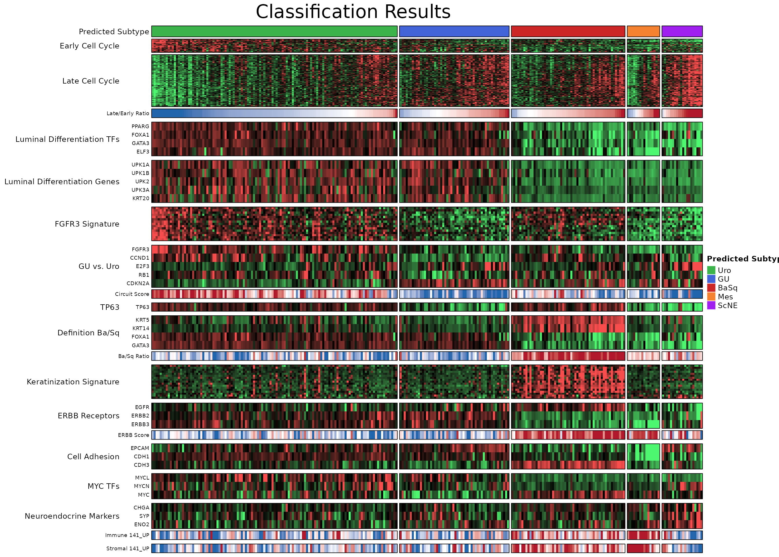
LundTaxR allows the user to generate sophisticated heatmaps that visualize both the classification results and 17 subtype defining molecular signatures. The plot_classification_heatmap() function creates a multi-layered visualization showing:

Sample classifications with color-coded subtype annotations
Molecular signatures subtype defining signatures, pathway activity scores and overall immune and stromal infiltration
Gene expression patterns for highlighting subtype-specific expression profiles
Prediction confidence reported subtype-specific scores for each sample

The heatmap automatically orders samples by subtype and within each subtype by prolfieration score, making it easy to identify patterns and validate classifications. You can choose between 5-class (Uro, GU, BaSq, Mes, ScNE) or 7-class (UroA, UroB, UroC, GU, BaSq, Mes, ScNE) annotation systems.

# Create a comprehensive classification heatmap
plot_classification_heatmap(
  these_predictions = sjodahl_classes,              # Classification results from classify_samples()
  subtype_annotation = "5_class",                   # Use 5-class system (Uro, GU, BaSq, Mes, ScNE)
  plot_scores = FALSE,                              # Hide individual prediction scores for cleaner view
  plot_title = "Classification Results",            # Custom title for the visualization
  show_ann_legend = TRUE,                           # Display subtype color legend
  ann_height = 0.5                                  # Compact annotation track height
)


# The function displays the heatmap directly in your R session
# To save the plot, add out_path and out_format parameters:
# plot_classification_heatmap(
#   these_predictions = sjodahl_classes,
#   subtype_annotation = "5_class", 
#   out_path = "results/",                          # Directory to save plot
#   out_format = "png",                             # File format (png or pdf)
#   plot_title = "Classification_Heatmap",
#   plot_width = 12,                                # Width in inches
#   plot_height = 8                                 # Height in inches
# )

The resulting heatmap provides a comprehensive overview of your classification results, with samples grouped by predicted subtype and colored according to the LundTax system. This visualization is essential for:

Quality assessment: Verify that samples cluster appropriately within subtypes
Pattern recognition: Identify molecular signatures that distinguish subtypes
Publication figures: Generate high-quality plots ready for publication
Result interpretation: Understand the biological basis of classifications

Visualizing Molecular Signatures with Signature Heatmaps

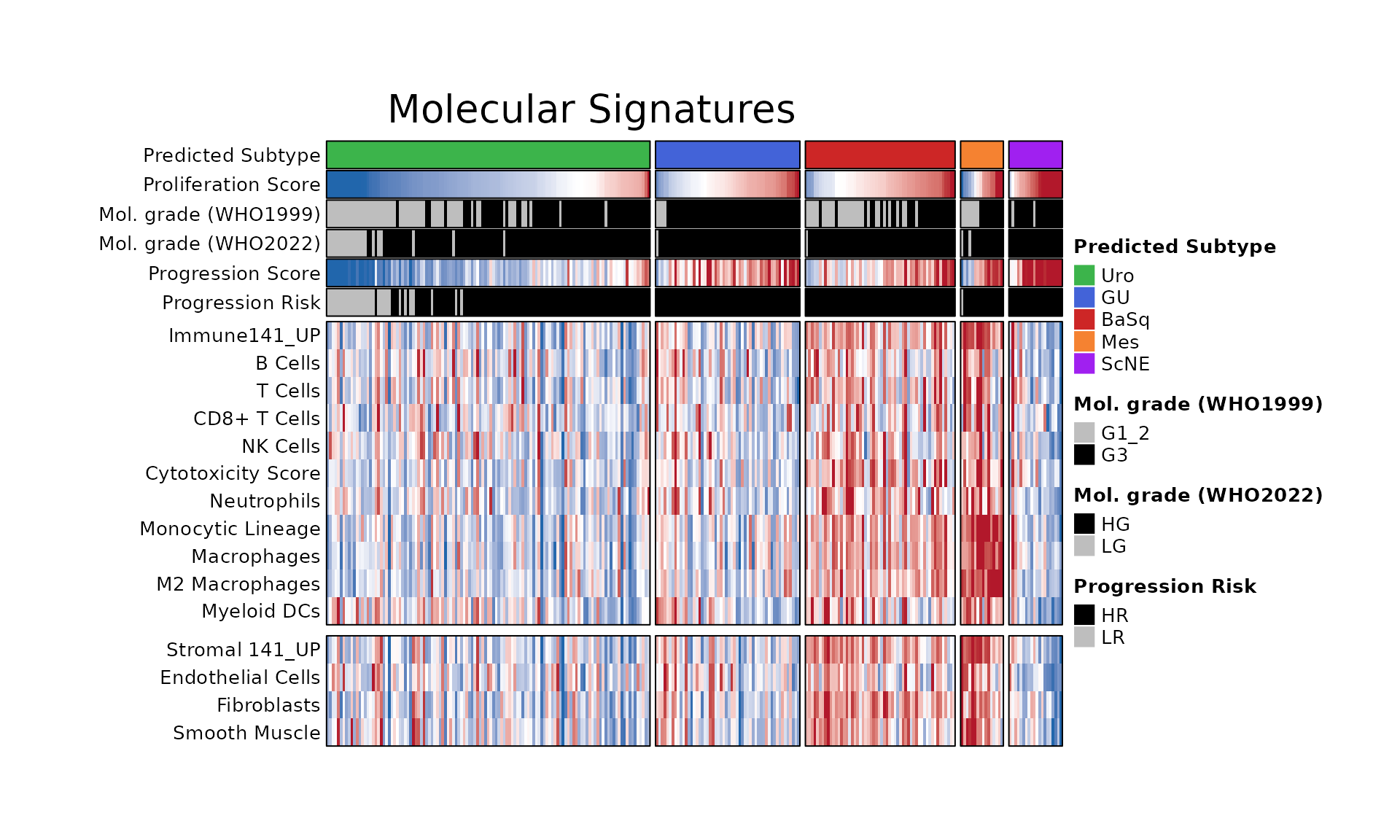
In addition to classification results, LundTaxR provides additional molecular profiling through signature scores that capture key biological processes. The plot_signatures_heatmap() function creates specialized visualizations focused on these molecular signatures, including:

Prognostic Signatures (molecular grading, proliferation, progression)
Immune infiltration scores (B cells, T cells, NK cells, dendritic cells, etc.)
Stromal content markers (CAFs, endothelial cells, smooth muscle)

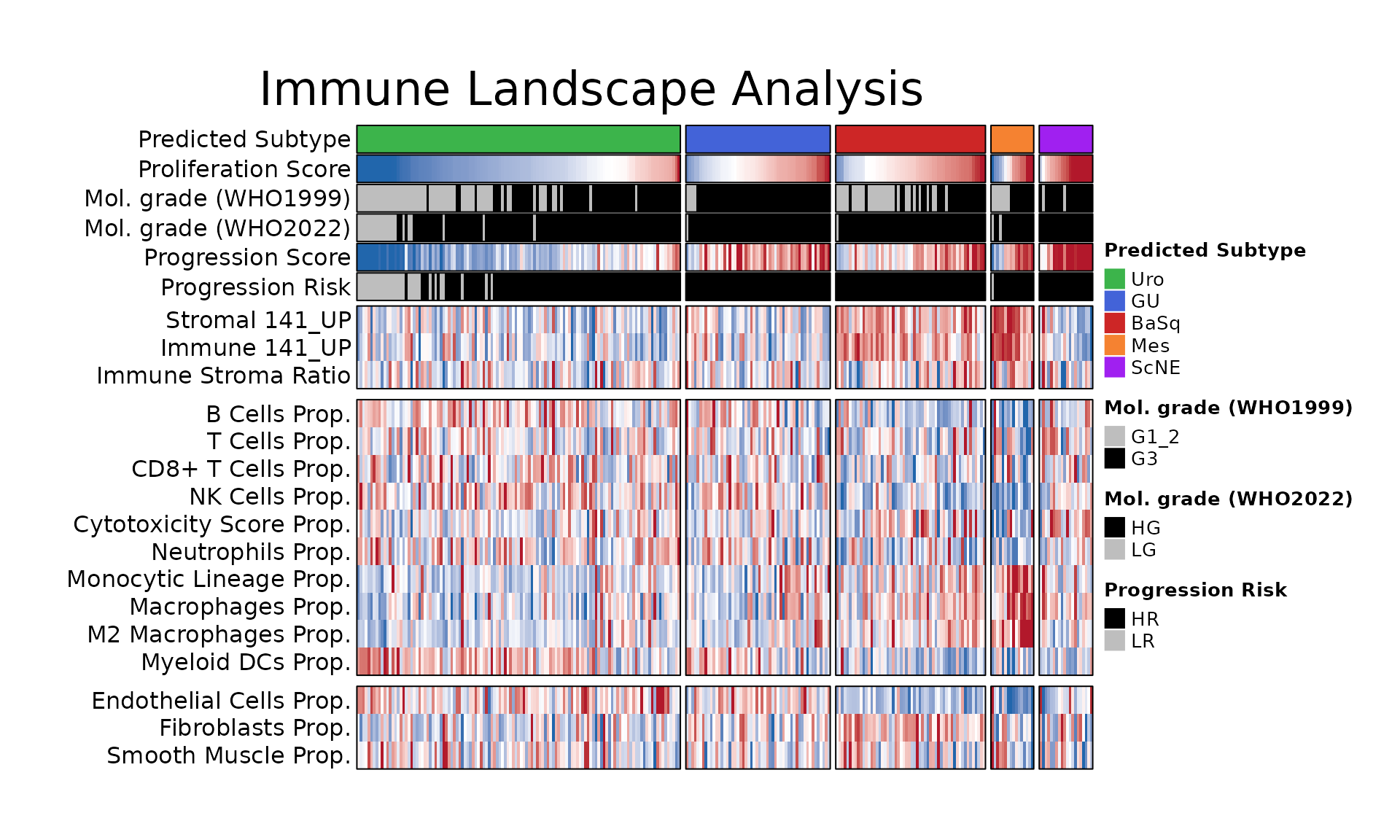
This visualization is particularly valuable for assessing tumor microenvironment signals that vary independently of the bladder cancer subtypes. The heatmap organizes samples by predicted subtype and displays signature scores as color-coded intensities, making it easy to identify variability within and across subtypes.

# Create a comprehensive molecular signatures heatmap
plot_signatures_heatmap(
  these_predictions = sjodahl_classes,              # Classification results with signature scores
  proportional_scores = FALSE,                      # Use raw signature scores (not proportions)
  plot_title = "Molecular Signatures",              # Custom title for the visualization
  plot_hm_legend = FALSE,                           # Display heatmap color scale legends
  plot_font_size = 10,                              # Font size for labels and annotations
)


# Alternative: Focus on immune signatures with proportional scoring
plot_signatures_heatmap(
  these_predictions = sjodahl_classes,
  proportional_scores = TRUE,                       # Convert scores to proportions (0-1 scale)
  plot_title = "Immune Landscape Analysis",
  plot_hm_legend = FALSE,
  plot_font_size = 12
)


# Save high-quality plot for publication
# plot_signatures_heatmap(
#   these_predictions = sjodahl_classes,
#   out_path = "figures/",                          # Directory to save plot
#   out_format = "pdf",                             # High-resolution PDF format
#   plot_title = "Molecular_Signatures_Heatmap",
#   plot_width = 14,                                # Width in inches for publication
#   plot_height = 10,                               # Height in inches
#   plot_font_size = 8                              # Smaller font for publication
# )

Understanding the Output

The signature heatmap reveals several key biological insights:

Subtype-specific patterns: Each molecular subtype shows distinct signature score profiles
Proliferation patterns: ScNE samples often display high proliferation scores
Immune microenvironment: Immune infiltration may vary dramatically between subtypes (e.g., high in Mes, low in UroA)
Stromal content: Mesenchymal subtypes typically show elevated stromal signatures
Clinical relevance: In NMIBC, progression risk scores help identify aggressive tumors within subtypes

This visualization complements the classification heatmap by visualizing additional key features of tumor biology, providing insights into bladder cancer heterogeneity beyond the cancer cell phenotype itself.

Adam Mattsson

2026-04-28