Advanced Classification Workflows

Introduction

This vignette demonstrates advanced parameter usage for the LundTax classifier, building upon the concepts introduced in the “Getting Started” guide. If you’re new to LundTaxR, we recommend starting with the basic tutorial first:

vignette("getting_started_with_LundTaxR", package = "LundTaxR")

Who This Guide Is For

This advanced guide is designed for researchers and bioinformaticians who want to:

Fine-tune classification parameters for optimal performance on their datasets
Understand the impact of preprocessing and imputation settings
Explore confidence scoring and progression risk thresholding
Build reproducible analytical pipelines for improved consistency in research

What You’ll Learn

Parameter optimization: Fine-tuning classification thresholds and confidence scores
Custom classifier settings: Adapting the algorithm for specific data characteristics
Performance evaluation: Assessing and improving classification accuracy
Handling edge cases: Dealing with ambiguous or low-quality samples

Prerequisites

Solid understanding of R programming and data manipulation
Experience with molecular profiling data (RNA-seq, microarrays)
Completed the “Getting Started with LundTaxR” tutorial

1. Advanced Classifier Configuration

The classify_samples() function offers numerous parameters that allow you to fine-tune the classification process for optimal performance on your specific datasets. Understanding these parameters and their interactions is crucial for achieving reliable and reproducible results.

1.1 Classification Thresholds and Confidence Scoring

The LundTaxR classifier uses a two-stage approach: first classifying samples into 5 main classes (Uro, GU, BaSq, Mes, ScNE), then further classifying Uro samples into the following subgroups: UroA, UroB, and UroC. For each sample, the output shows the normalized subtype scores for each subtype, that sums to 1 for the main subtypes and within the Uro classes.

# Load example data
data("sjodahl_2017")

# Basic classification with default parameters
basic_results <- classify_samples(
  this_data = sjodahl_2017,
  verbose = TRUE
)
#> 
#> ============================================================
#>   LUND TAXONOMY CLASSIFIER
#> ============================================================
#>   Data Check: The data is likely log2-transformed. The range 
#>   and distribution are consistent with log2-transformed data. 
#>   Input samples: 267 
#>   Input genes: 15697 
#>   Gene ID format: hgnc_symbol
#> ============================================================
#>   SUBTYPE CLASSIFICATION
#> ============================================================
#>   1. Predicting 5-class subtypes
#> ------------------------------------------------------------
#>   2. Subclassifying Uro samples
#> ============================================================
#>   SIGNATURE CALCULATION
#> ============================================================
#>   1. Calculating Proliferation Score
#> ------------------------------------------------------------
#>   2. Calculating Progression Score
#> ------------------------------------------------------------
#>   3. Applying Grade Predictor (WHO1999):
#>          Total rules in classifier: 283
#>          Rules with both genes present: 246
#>          Rules removed: 37
#>          Samples to score: 267
#>          Grade threshold: 0.5
#>          Grade labels: G1_2 / G3
#> ------------------------------------------------------------
#>   4. Applying Grade Predictor (WHO2022):
#>          Total rules in classifier: 140
#>          Rules with both genes present: 119
#>          Rules removed: 21
#>          Samples to score: 267
#>          Grade threshold: 0.5
#>          Grade labels: LG / HG
#> ------------------------------------------------------------
#>   5. Calculating Immune Signature Scores
#> ------------------------------------------------------------
#>   6. Calculating Stromal and Immune Composite Scores
#> ------------------------------------------------------------
#>   7. Merging Scores
#> ============================================================
#>   CLASSIFICATION COMPLETE
#> ============================================================
#>     UroA: 43 samples
#>     UroB: 27 samples
#>     UroC: 51 samples
#>     GU: 54 samples
#>     BaSq: 56 samples
#>     Mes: 16 samples
#>     ScNE: 20 samples
#> ------------------------------------------------------------

# Examine the prediction confidence scores
head(basic_results$subtype_scores)
#>          Uro   UroA   UroB   UroC     GU   BaSq    Mes   ScNE
#> 1.CEL 0.9924 0.9350 0.0048 0.0602 0.0072 0.0004 0.0000 0.0000
#> 2.CEL 0.0016     NA     NA     NA 0.0052 0.0054 0.9804 0.0074
#> 3.CEL 0.0682     NA     NA     NA 0.7754 0.0834 0.0390 0.0340
#> 4.CEL 0.9930 0.9334 0.0028 0.0638 0.0066 0.0004 0.0000 0.0000
#> 5.CEL 0.9808 0.0058 0.9878 0.0064 0.0076 0.0090 0.0006 0.0020
#> 6.CEL 0.0082     NA     NA     NA 0.9890 0.0002 0.0004 0.0022
#>       prediction_delta_5_class prediction_delta_7_class
#> 1.CEL                   0.9852                   0.8748
#> 2.CEL                   0.9730                       NA
#> 3.CEL                   0.6920                       NA
#> 4.CEL                   0.9864                   0.8696
#> 5.CEL                   0.9718                   0.9814
#> 6.CEL                   0.9808                       NA
#>       prediction_delta_collapsed
#> 1.CEL                     0.8748
#> 2.CEL                     0.9730
#> 3.CEL                     0.6920
#> 4.CEL                     0.8696
#> 5.CEL                     0.9814
#> 6.CEL                     0.9808

The prediction_delta column shows the confidence of each classification - the difference between the highest and second-highest prediction scores. Higher delta values indicate more confident predictions.

# Analyze prediction confidence
confidence_summary <- data.frame(
  sample = names(basic_results$predictions_7classes),
  subtype_7c = basic_results$predictions_7classes,
  subtype_5c = basic_results$predictions_5classes,
  confidence = basic_results$subtype_scores[, "prediction_delta_5_class"]
)

# Identify low-confidence predictions
low_confidence <- confidence_summary[confidence_summary$confidence < 0.05, ]
print(paste("Samples with low confidence (delta < 0.05):", nrow(low_confidence)))
#> [1] "Samples with low confidence (delta < 0.05): 0"

# Distribution of confidence scores by subtype
library(dplyr)
confidence_by_subtype <- confidence_summary %>%
  group_by(subtype_7c) %>%
  summarise(
    mean_confidence = mean(confidence, na.rm = TRUE),
    median_confidence = median(confidence, na.rm = TRUE),
    min_confidence = min(confidence, na.rm = TRUE),
    .groups = 'drop'
  )
print(confidence_by_subtype)
#> # A tibble: 7 × 4
#>   subtype_7c mean_confidence median_confidence min_confidence
#>   <chr>                <dbl>             <dbl>          <dbl>
#> 1 BaSq                 0.942             0.984          0.650
#> 2 GU                   0.878             0.926          0.573
#> 3 Mes                  0.901             0.956          0.647
#> 4 ScNE                 0.897             0.894          0.685
#> 5 UroA                 0.983             0.998          0.717
#> 6 UroB                 0.926             0.98           0.695
#> 7 UroC                 0.939             0.969          0.635

1.2 Data Preprocessing Parameters

Log Transformation Control

LundTaxR automatically detects whether your data is log2-transformed, but you can override this behavior. Note: Log2 transformation primarily affects signature score calculations, not the classifier predictions themselves.

⚠️ CRITICAL: Signature score calculations require log2-transformed values. If your input data is already log2-transformed and you set log_transform = TRUE, the signature scores will be calculated on double-logged data, leading to incorrect results. Conversely, if your data is raw (non-logged) and you set log_transform = FALSE, signature scores will be calculated on untransformed data, which is also incorrect.

# Example with already log-transformed data (like sjodahl_2017)
# Setting log_transform = TRUE would cause double-logging
double_logged_results <- classify_samples(
  this_data = sjodahl_2017,
  log_transform = TRUE,  # INCORRECT: causes double log2 transformation
  verbose = FALSE
)

# Correct approach for already log-transformed data
correct_results <- classify_samples(
  this_data = sjodahl_2017,
  log_transform = FALSE, # CORRECT: data is already log2-transformed
  verbose = FALSE
)

# Compare classifier predictions (should be identical)
identical(basic_results$predictions_7classes, correct_results$predictions_7classes)
#> [1] TRUE
identical(basic_results$predictions_7classes, double_logged_results$predictions_7classes)
#> [1] TRUE

# Compare signature scores - double logging severely distorts scores
score_comparison <- data.frame(
  sample = rownames(basic_results$scores)[1:5], # Show first 5 samples
  correct_immune = correct_results$scores$immune141_up[1:5],
  double_logged_immune = double_logged_results$scores$immune141_up[1:5],
  ratio = correct_results$scores$immune141_up[1:5] / double_logged_results$scores$immune141_up[1:5]
)
print(score_comparison)
#>   sample correct_immune double_logged_immune     ratio
#> 1  1.CEL       4.274890             4.722811 0.9051578
#> 2  2.CEL       5.356312             5.208732 1.0283332
#> 3  3.CEL       5.500902             5.273202 1.0431805
#> 4  4.CEL       4.366632             4.772984 0.9148641
#> 5  5.CEL       4.527595             4.850548 0.9334192

# The impact is substantial
cat("Mean immune score - Correct:", round(mean(correct_results$scores$immune141_up), 3), "\n")
#> Mean immune score - Correct: 4.875
cat("Mean immune score - Double-logged:", round(mean(double_logged_results$scores$immune141_up), 3), "\n")
#> Mean immune score - Double-logged: 5.002

Best Practice Guidelines: - For raw count data (RNA-seq, microarray): Set log_transform = TRUE - For already log-transformed data: Set log_transform = FALSE - When uncertain: Let LundTaxR auto-detect (recommended default behavior) - Always validate: Check that signature score ranges are reasonable for your data type

Score Adjustment and Normalization

The adjustment parameters are crucial for signature score calculations but do not affect the classifier subtype predictions. These parameters control how signature scores are normalized based on stable reference genes:

# Classification without score adjustment
no_adjustment <- classify_samples(
  this_data = sjodahl_2017,
  adjust = FALSE,  # Skip normalization step for signatures
  verbose = FALSE
)

# Custom adjustment factor (default is 5.1431)
custom_adjustment <- classify_samples(
  this_data = sjodahl_2017,
  adjust = TRUE,
  adj_factor = 3.0,  # Lower factor = more conservative signature scores
  verbose = FALSE
)

# Classifier predictions remain identical
identical(basic_results$predictions_7classes, no_adjustment$predictions_7classes)
#> [1] TRUE
identical(basic_results$predictions_7classes, custom_adjustment$predictions_7classes)
#> [1] TRUE

# But signature scores differ significantly
signature_comparison <- data.frame(
  sample = rownames(basic_results$scores),
  default_luminal = basic_results$scores$b_cells,
  no_adj_luminal = no_adjustment$scores$b_cells,
  custom_adj_luminal = custom_adjustment$scores$b_cells
)

# Summary statistics show the impact on signature scores
summary(signature_comparison[, -1])
#>  default_luminal no_adj_luminal  custom_adj_luminal
#>  Min.   :3.069   Min.   :4.336   Min.   :1.790     
#>  1st Qu.:3.431   1st Qu.:4.678   1st Qu.:2.001     
#>  Median :3.616   Median :4.836   Median :2.109     
#>  Mean   :3.655   Mean   :4.897   Mean   :2.132     
#>  3rd Qu.:3.829   3rd Qu.:5.033   3rd Qu.:2.233     
#>  Max.   :4.683   Max.   :6.147   Max.   :2.732

1.3 Missing Data Handling and Sample Rejection

The LundTaxR classifier always assigns a subtype to every sample, but the imputation parameters control how missing gene expression data is handled during the classification process:

# Strict imputation settings (conservative approach)
strict_imputation <- classify_samples(
  this_data = sjodahl_2017,
  impute = TRUE,
  impute_kNN = 3,        # Use only 3 nearest neighbors
  impute_reject = 0.4,   # Reject samples with >40% missing classification rules
  verbose = FALSE
)

# Lenient imputation settings
lenient_imputation <- classify_samples(
  this_data = sjodahl_2017,
  impute = TRUE,
  impute_kNN = 10,       # Use 10 nearest neighbors
  impute_reject = 0.8,   # Accept samples with up to 80% missing classification rules
  verbose = FALSE
)

# All approaches classify the same number of samples
comparison <- data.frame(
  method = c("Default", "Strict", "Lenient"),
  samples_classified = c(
    length(basic_results$predictions_7classes),
    length(strict_imputation$predictions_7classes),
    length(lenient_imputation$predictions_7classes)
  ),
  samples_input = rep(ncol(sjodahl_2017), 3)
)
print(comparison)
#>    method samples_classified samples_input
#> 1 Default                267           267
#> 2  Strict                267           267
#> 3 Lenient                267           267

Key Point: The impute_reject threshold determines when a sample has too much missing data for reliable classification, but in practice, the classifier will still assign a subtype.

1.4 Performance Optimization

For large datasets or when you only need classification results, you can optimize performance:

# Minimal output - only subtypes (fastest)
minimal_results <- classify_samples(
  this_data = sjodahl_2017,
  subtype_only = TRUE,      # Skip signature score calculations
  include_data = FALSE,     # Don't include input data in output
  include_pred_scores = FALSE,  # Skip prediction score matrix
  verbose = FALSE
)

# Check what's returned
str(minimal_results)
#> List of 2
#>  $ predictions_7classes: Named chr [1:267] "UroA" "Mes" "GU" "UroA" ...
#>   ..- attr(*, "names")= chr [1:267] "1.CEL" "2.CEL" "3.CEL" "4.CEL" ...
#>  $ predictions_5classes: Named chr [1:267] "Uro" "Mes" "GU" "Uro" ...
#>   ..- attr(*, "names")= chr [1:267] "1.CEL" "2.CEL" "3.CEL" "4.CEL" ...

# Timing comparison for large datasets
system.time({
  full_analysis <- classify_samples(sjodahl_2017, verbose = FALSE)
})
#>    user  system elapsed 
#>   5.582   0.046   5.379

system.time({
  minimal_analysis <- classify_samples(
    sjodahl_2017, 
    subtype_only = TRUE, 
    include_pred_scores = FALSE,
    verbose = FALSE
  )
})
#>    user  system elapsed 
#>   0.895   0.023   0.661

1.5 Custom Progression Risk Thresholds

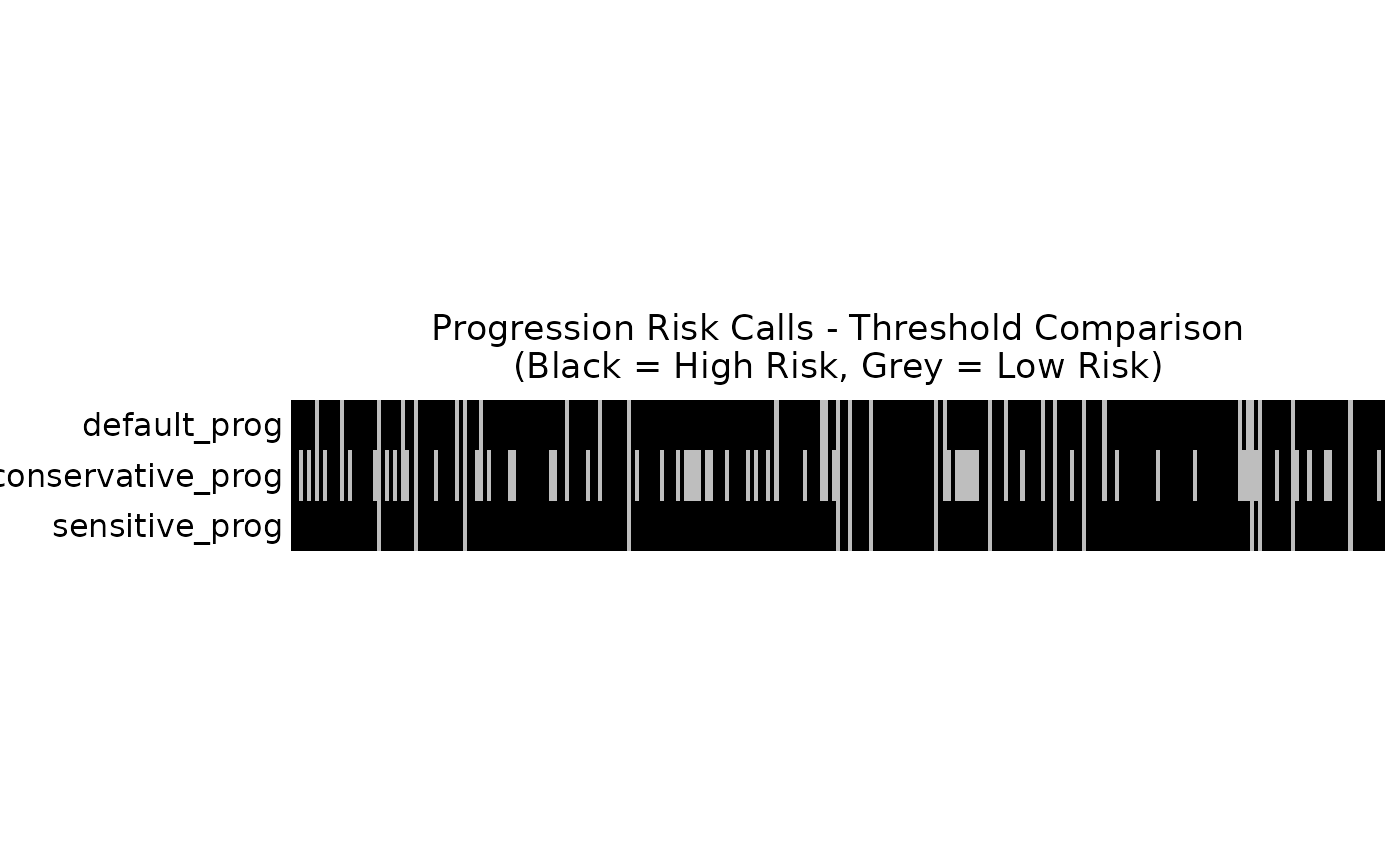
The classifier includes a progression risk score, a continuous score ranging from 0-1, that can be customized based on your clinical context. The default cutoff 0.56 classifies samples above the set threshold into High Risk (HR) and below the threshold to Low Risk (LR). You can adjust this threshold to be more conservative or sensitive. Note: The example dataset primarily consists of muscle-invasive bladder cancer (MIBC) cases, which represent tumors that have already progressed beyond the muscle layer. The progression risk score displayed here was originally developed and validated for non-muscle-invasive bladder cancer (NMIBC) patients to predict their probability of future progression to muscle-invasive disease.

# Conservative progression threshold
conservative_prog <- classify_samples(
  this_data = sjodahl_2017,
  threshold_progression = 0.7,  # Higher threshold (more specific)
  verbose = FALSE
)

# Sensitive progression threshold  
sensitive_prog <- classify_samples(
  this_data = sjodahl_2017,
  threshold_progression = 0.5,  # Lower threshold (more sensitive)
  verbose = FALSE
)

# Compare progression classifications
prog_comparison <- data.frame(
  sample = names(basic_results$predictions_7classes),
  default_prog = basic_results$scores$progression_risk,
  conservative_prog = conservative_prog$scores$progression_risk,
  sensitive_prog = sensitive_prog$scores$progression_risk
)

# Convert to matrix for heatmap
prog_mat <- as.matrix(prog_comparison[, c("default_prog", "conservative_prog", "sensitive_prog")])
rownames(prog_mat) <- prog_comparison$sample

# Map HR/LR to colors
prog_colors <- c("HR" = "black", "LR" = "grey")

Heatmap(
  t(prog_mat),
  name = "Progression",
  col = prog_colors,
  cluster_rows = FALSE,
  cluster_columns = FALSE,
  show_row_names = TRUE,
  show_column_names = FALSE,
  height = unit(2, "cm"),
  column_title = "Progression Risk Calls - Threshold Comparison\n(Black = High Risk, Grey = Low Risk)",
  show_heatmap_legend = FALSE,
  row_names_side = "left"
)

1.6 Quality Control and Validation

Always examine the missing genes information and prediction quality:

# Examine missing genes
missing_info <- basic_results$na_genes
print(paste("Genes missing from input data:", nrow(missing_info)))
#> [1] "Genes missing from input data: 67"
if(nrow(missing_info) > 0) {
  head(missing_info)
}
#>      genes     signature process
#> 1   NUSAP1 proliferation      up
#> 2     PRC1 proliferation      up
#> 3   FAM72D proliferation      up
#> 4   FAM72A proliferation      up
#> 5 RNASEH2A proliferation      up
#> 6    POLA2 proliferation      up

# Identify samples with potential quality issues
quality_flags <- data.frame(
  sample = names(basic_results$predictions_7classes),
  confidence = basic_results$subtype_scores[, "prediction_delta_5_class"],
  quality_flag = basic_results$subtype_scores[, "prediction_delta_5_class"] < 0.05
)

flagged_samples <- quality_flags[quality_flags$quality_flag, ]
if(nrow(flagged_samples) > 0) {
  print("Samples flagged for low confidence:")
  head(flagged_samples)
}

Key Takeaways

Start with default parameters and adjust based on your data characteristics
Monitor prediction confidence using the prediction_delta scores
Validate imputation settings with your dataset’s missing data patterns
Consider performance optimization for large-scale analyses
Always examine quality control metrics before downstream analysis

Adam Mattsson

2026-04-28